Institute of Actuaries of India 2006 CT4 Models Core Technical - Question Paper
Faculty of Actuaries Institute of Actuaries
6 September 2006 (am)
Subject CT4 Models Core Technical
Time allowed: Three hours INSTRUCTIONS TO THE CANDIDATE
1. Enter all the candidate and examination details as requested on the front of your answer booklet.
2. You must not start writing your answers in the booklet until instructed to do so by the supervisor.
3. Mark allocations are shown in brackets.
4. Attempt all 12 questions, beginning your answer to each question on a separate sheet.
5. Candidates should show calculations where this is appropriate.
Graph paper is not required for this paper.
A T THE END OF THE EXAMINA TION
Hand in BOTH your answer booklet, with any additional sheets firmly attached, and this question paper.
In addition to this paper you should have available the 2002 edition ofthe Formulae and Tables and your own electronic calculator.
A1 A manufacturer uses a test rig to estimate the failure rate in a batch of electronic components. The rig holds 100 components and is designed to detect when a component fails, at which point it immediately replaces the component with another from the same batch. The following are recorded for each of the n components used in the test (i = 1,2,... ,n):
Si = time at which component i placed on the rig tj = time at which component i removed from rig
[l Component removed due tofailure 1 [ 0 Component working at end of test period
The test rig was fully loaded and was run for two years continuously.
You should assume that the force of failure, \i, of a component is constant and component failures are independent.
(i) Show that the contribution to the likelihood from component i is:
exp(-(j. (ti-s-|aii [2]
(ii) Derive the maximum likelihood estimator for p. [4]
[Total 6]
A2 The price of a stock can either take a value above a certain point (state A), or take a value below that point (state B). Assume that the evolution of the stock price in time can be modelled by a two-state Markov jump process with homogeneous transition rates o ab = , ba = P.
The process starts in state A at t = 0 and time is measured in weeks.
(i) Write down the generator matrix of the Markov jump process. [1]
(ii) State the distribution of the holding time in each of states A and B. [1]
(iii) If a = 3, find the value of t such that the probability that no transition to state B has occurred until time t is 0.2. [2]
(iv) Assuming all the information about the price of the stock is available for a time interval [0, T], explain how the model parameters a and p can be estimated from the available data. [2]
(v) State what you would test to determine whether the data support the assumption of a two-state Markov jump process model for the stock price. [1]
[Total 7]
(a) a Poisson process
(b) a compound Poisson process; and
(c) a general random walk
(ii) For each of the processes in (i), state whether it operates in continuous or discrete time and whether it has a continuous or discrete state space. [2]
(iii) For each of the processes in (i), describe one practical situation in which an actuary could use such a process to model a real world phenomenon. [3]
[Total 8]
A4 The credit-worthiness of debt issued by companies is assessed at the end of each year by a credit rating agency. The ratings are A (the most credit-worthy), B and D (debt defaulted). Historic evidence supports the view that the credit rating of a debt can be modelled as a Markov chain with one-year transition matrix
|
X = |
|
0.1 1 |
(i) Determine the probability that a company rated A will never be rated B in the future. [2]
(ii) (a) Calculate the second order transition probabilities of the Markov chain.
(b) Hence calculate the expected number of defaults within the next two
years from a group of 100 companies, all initially rated A. [2]
The manager of a portfolio investing in company debt follows a downgrade trigger strategy. Under this strategy, any debt in a company whose rating has fallen to B at the end of a year is sold and replaced with debt in an A-rated company.
(iii) Calculate the expected number of defaults for this investment manager over the next two years, given that the portfolio initially consists of 100 A-rated bonds. [2]
(iv) Comment on the suggestion that the downgrade trigger strategy will improve the return on the portfolio. [2]
[Total 8]
A5 A motor insurance company wishes to estimate the proportion of policyholders who
make at least one claim within a year. From historical data, the company believes that the probability a policyholder makes a claim in any given year depends on the number of claims the policyholder made in the previous two years. In particular:
the probability that a policyholder who had claims in both previous years will make a claim in the current year is 0.25
the probability that a policyholder who had claims in one of the previous two years will make a claim in the current year is 0.15; and
the probability that a policyholder who had no claims in the previous two years will make a claim in the current year is 0.1
(i) Construct this as a Markov chain model, identifying clearly the states of the chain. [2]
(ii) Write down the transition matrix of the chain. [1]
(iii) Explain why this Markov chain will converge to a stationary distribution. [2]
(iv) Calculate the proportion of policyholders who, in the long run, make at least one claim at a given year. [4]
[Total 9]
A6 (i) Explain the difference between a time-homogeneous and a time-
inhomogeneous Poisson process. [1]
An insurance company assumes that the arrival of motor insurance claims follows an inhomogeneous Poisson process.
Data on claim arrival times are available for several consecutive years.
(ii) (a) Describe the main steps in the verification of the companys
assumption.
(b) State one statistical test that can be used to test the validity of the assumption.
[3]
(iii) The company concludes that an inhomogeneous Poisson process with rate A,(t)=3 + cos(2n;t) is a suitable fit to the claim data (where tis measured in years).
(a) Comment on the suitability of this transition rate for motor insurance claims.
(b) Write down the Kolmogorov forward equations for P0 j(s, t) .
(c) Verify that these equations are satisfied by:
P (sA ( f(S, t))7eXP f(S, t))
P0 j(s, r) - " j!
for some f(s,t) which you should identify.
[Note that Jcos xdx =sin x.]
(d) Comment on the form of the solution compared with the case where k is constant.
[Total 12]
B1 Calculate 0 25 p80 and 0 25 p80 5 using the ELT15 (Females) mortality table and
assuming a uniform distribution of deaths.
B2 A national mortality investigation is carried out over the calendar years 2002, 2003 and 2004. Data are collected from a number of insurance companies.
Deaths during the period of the investigation, 0x, are classified by age nearest at death.
Each insurance company provides details of the number of in-force policies on 1 January 2002, 2003, 2004 and 2005, where policyholders are classified by age nearest birthday, Pt).
(i) (a) State the rate year implied by the classification of deaths.
(b) State the ages of the lives at the start of the rate interval.
(ii) Derive an expression for the exposed to risk, in terms of Px(t), which may be used to estimate the force of mortality in year t at each age. State any
assumptions you make.
[3]
(iii) Describe how your answer to (ii) would change if the census information
provided by some companies was P* ( t), the number of in-force policies on
1 January each year, where policyholders are classified by age last birthday.
[3]
[Total 7]
B3 An investigation was undertaken into the effect of a new treatment on the survival times of cancer patients. Two groups of patients were identified. One group was given the new treatment and the other an existing treatment.
The following model was considered:
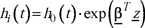
where: hf) is the hazard at time t, where t is the time since the start of treatment h (t) is the baseline hazard at time t
z is a vector of covariates such that:
z1 = sex (a categorical variable with 0 = female, 1 = male)
z2 = treatment (a categorical variable with 0 = existing treatment,
1 = new treatment)
and pis a vector of parameters, ((3b |32 ).
A the risk of death for a male patient is 1.02 times that of a female patient; and
B the risk of death for a patient given the existing treatment is 1.05 times that for a patient given the new treatment
(i) Estimate the value of the parameters and P2 . [3]
(ii) Estimate the ratio by which the risk of death for a male patient who has been given the new treatment is greater or less than that for a female patient given the existing treatment. [2]
(iii) Determine, in terms of the baseline hazard only, the probability that a male patient will die within 3 years of receiving the new treatment. [2]
[Total 7]
B4 An investigation took place into the mortality of persons between exact ages 60 and 61 years. The table below gives an extract from the results. For each person it gives the age at which they were first observed, the age at which they ceased to be observed and the reason for their departure from observation.
|
Person Age at entry Age at exit Reason for exit | ||||||||||||||||||||||||||||||||||||||||||||||||||||||||||||||||||
|
(i) Estimate q60 using the Binomial model. [5]
(ii) List the strengths and weaknesses of the Binomial model for the estimation of empirical mortality rates, compared with the Poisson and two-state models.
[3]
[Total 8]
B5 A life insurance company has carried out a mortality investigation. It followed a sample of independent policyholders aged between 50 and 55 years. Policyholders were followed from their 50th birthday until they died, they withdrew from the investigation while still alive, or they celebrated their 55th birthday (whichever of these events occurred first).
(i) Describe the censoring that is present in this investigation. [2]
An extract from the data for 12 policyholders is shown in the table below.
|
Policyholder Last age at which Outcome policyholder was observed | |||||||||||||||||||||||||||||||||||||||
|
(ii) Calculate the Nelson-Aalen estimate of the survival function. [5]
(iii) Sketch on a suitably labelled graph the Nelson-Aalen estimate of the survival function. [2]
[Total 9]
B6 (i) (a) Describe the general form of the polynomial formula used to graduate the most recent standard tables produced for use by UK life insurance companies.
(b) Show how the Gompertz and Makeham formulae arise as special cases of this formula.
[3]
(ii) An investigation was undertaken of the mortality of persons aged between 40 and 75 years who are known to be suffering from a degenerative disease. It is suggested that the crude estimates be graduated using the formula:
2
f
+ b2
1 ' x+
2 >
1
x+ 2
o
2
(a) Explain why this might be a sensible formula to choose for this class of lives.
(b) Suggest two techniques which can be used to perform the graduation.
[3]
(iii) The table below shows the crude and graduated mortality rates for part of the relevant age range, together with the exposed to risk at each age and the standardised deviation at each age.
Age last Graduated birthday force of mortality
Crude force of mortality
Standardised deviation
Exposed to risk
c
Ax+1/2 Mx+1/2
o
Mx+1/2
c
x
Mx+1/2
z =-
|
o | ||||||||||||||||||||||||||||||||||||||||
|
ec
Mx+12
Test this graduation for:
(a) overall goodness-of-fit
(b) bias; and
(c) the existence of individual ages at which the graduated rates depart to a substantial degree from the observed rates
[9]
[Total 15]
CT4 S20069
|
Attachment: |
| Earning: Approval pending. |